Tree Recursion
Another common pattern of computation is called tree recursion. As an example, consider computing the sequence of Fibonacci numbers, in which each number is the sum of the preceding two:

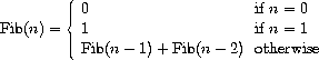
In general, the Fibonacci numbers can be defined by the rule
We can immediately translate this definition into a recursive procedure for computing Fibonacci numbers:
(define (fib n)
  (cond ((= n 0) 0)
        ((= n 1) 1)
        (else (+ (fib (- n 1))
                 (fib (- n 2))))))
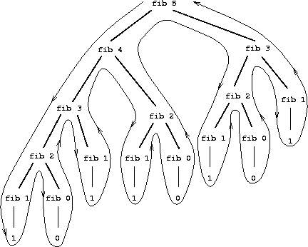
Figure 1.5:
The tree-recursive process generated in computing (fib 5).
Consider the pattern of this computation. To compute (fib 5), we compute (fib 4) and (fib 3). To compute (fib 4), we compute (fib 3) and (fib 2). In general, the evolved process looks like a tree, as shown in figure 1.5. Notice that the branches split into two at each level (except at the bottom); this reflects the fact that the fib procedure calls itself twice each time it is invoked.
This procedure is instructive as a prototypical tree recursion, but it is a terrible way to compute Fibonacci numbers because it does so much redundant computation. Notice in figure 1.5 that the entire computation of (fib 3) -- almost half the work -- is duplicated. In fact, it is not hard to show that the number of times the procedure will compute (fib 1) or (fib 0) (the number of leaves in the above tree, in general) is precisely Fib(n + 1). To get an idea of how bad this is, one can show that the value of Fib(n) grows exponentially with n. More precisely (see exercise 1.13), Fib(n) is the closest integer to  n /
n / 5, where
is the golden ratio, which satisfies the equation

Thus, the process uses a number of steps that grows exponentially with the input. On the other hand, the space required grows only linearly with the input, because we need keep track only of which nodes are above us in the tree at any point in the computation. In general, the number of steps required by a tree-recursive process will be proportional to the number of nodes in the tree, while the space required will be proportional to the maximum depth of the tree.
We can also formulate an iterative process for computing the Fibonacci numbers. The idea is to use a pair of integers a and b, initialized to Fib(1) = 1 and Fib(0) = 0, and to repeatedly apply the simultaneous transformations

It is not hard to show that, after applying this transformation n times, a and b will be equal, respectively, to Fib(n + 1) and Fib(n). Thus, we can compute Fibonacci numbers iteratively using the procedure
(define (fib n)
  (fib-iter 1 0 n))

(define (fib-iter a b count)
  (if (= count 0)
      b
      (fib-iter (+ a b) a (- count 1))))
This second method for computing Fib(n) is a linear iteration. The difference in number of steps required by the two methods -- one linear in n, one growing as fast as Fib(n) itself -- is enormous, even for small inputs.
One should not conclude from this that tree-recursive processes are useless. When we consider processes that operate on hierarchically structured data rather than numbers, we will find that tree recursion is a natural and powerful tool.31 But even in numerical operations, tree-recursive processes can be useful in helping us to understand and design programs. For instance, although the first fib procedure is much less efficient than the second one, it is more straightforward, being little more than a translation into Lisp of the definition of the Fibonacci sequence. To formulate the iterative algorithm required noticing that the computation could be recast as an iteration with three state variables.
Example: Counting change
It takes only a bit of cleverness to come up with the iterative Fibonacci algorithm. In contrast, consider the following problem: How many different ways can we make change of $ 1.00, given half-dollars, quarters, dimes, nickels, and pennies? More generally, can we write a procedure to compute the number of ways to change any given amount of money?
This problem has a simple solution as a recursive procedure. Suppose we think of the types of coins available as arranged in some order. Then the following relation holds:
The number of ways to change amount a using n kinds of coins equals
- the number of ways to change amount a using all but the first kind of coin, plus
- the number of ways to change amount a - d using all n kinds of coins, where d is the denomination of the first kind of coin.
To see why this is true, observe that the ways to make change can be divided into two groups: those that do not use any of the first kind of coin, and those that do. Therefore, the total number of ways to make change for some amount is equal to the number of ways to make change for the amount without using any of the first kind of coin, plus the number of ways to make change assuming that we do use the first kind of coin. But the latter number is equal to the number of ways to make change for the amount that remains after using a coin of the first kind.
Thus, we can recursively reduce the problem of changing a given amount to the problem of changing smaller amounts using fewer kinds of coins. Consider this reduction rule carefully, and convince yourself that we can use it to describe an algorithm if we specify the following degenerate cases:32
- If a is exactly 0, we should count that as 1 way to make change.
- If a is less than 0, we should count that as 0 ways to make change.
- If n is 0, we should count that as 0 ways to make change.
We can easily translate this description into a recursive procedure:
(define (count-change amount)
  (cc amount 5))
(define (cc amount kinds-of-coins)
  (cond ((= amount 0) 1)
        ((or (< amount 0) (= kinds-of-coins 0)) 0)
        (else (+ (cc amount
                     (- kinds-of-coins 1))
                 (cc (- amount
                        (first-denomination kinds-of-coins))
                     kinds-of-coins)))))
(define (first-denomination kinds-of-coins)
  (cond ((= kinds-of-coins 1) 1)
        ((= kinds-of-coins 2) 5)
        ((= kinds-of-coins 3) 10)
        ((= kinds-of-coins 4) 25)
        ((= kinds-of-coins 5) 50)))
(The first-denomination procedure takes as input the number of kinds of coins available and returns the denomination of the first kind. Here we are thinking of the coins as arranged in order from largest to smallest, but any order would do as well.) We can now answer our original question about changing a dollar:
(count-change 100)
292
Count-change generates a tree-recursive process with redundancies similar to those in our first implementation of fib. (It will take quite a while for that 292 to be computed.) On the other hand, it is not obvious how to design a better algorithm for computing the result, and we leave this problem as a challenge. The observation that a tree-recursive process may be highly inefficient but often easy to specify and understand has led people to propose that one could get the best of both worlds by designing a "smart compiler" that could transform tree-recursive procedures into more efficient procedures that compute the same result.33
A function f is defined by the rule that f(n) = n if n<3 and f(n) = f(n - 1) + 2f(n - 2) + 3f(n - 3) if n> 3. Write a procedure that computes f by means of a recursive process. Write a procedure that computes f by means of an iterative process.
Exercise 1.12The following pattern of numbers is called Pascal's triangle.
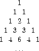
The numbers at the edge of the triangle are all 1, and each number inside the triangle is the sum of the two numbers above it.34 Write a procedure that computes elements of Pascal's triangle by means of a recursive process.
Exercise 1.13Prove that Fib(n) is the closest integer to n/5, where = (1 + 5)/2. Hint: Let  = (1 - 5)/2. Use induction and the definition of the Fibonacci numbers (see section 1.2.2) to prove that Fib(n) = (n - n)/5.
31An example of this was hinted at in section 1.1.3: The interpreter itself evaluates expressions using a tree-recursive process.
32For example, work through in detail how the reduction rule applies to the problem of making change for 10 cents using pennies and nickels.
33One approach to coping with redundant computations is to arrange matters so that we automatically construct a table of values as they are computed. Each time we are asked to apply the procedure to some argument, we first look to see if the value is already stored in the table, in which case we avoid performing the redundant computation. This strategy, known as tabulation or memoization, can be implemented in a straightforward way. Tabulation can sometimes be used to transform processes that require an exponential number of steps (such as count-change) into processes whose space and time requirements grow linearly with the input. See exercise 3.27.
34The elements of Pascal's triangle are called the binomial coefficients, because the nth row consists of the coefficients of the terms in the expansion of (x + y)n. This pattern for computing the coefficients appeared in Blaise Pascal's 1653 seminal work on probability theory, Traité du triangle arithmétique. According to Knuth (1973), the same pattern appears in the Szu-yuen Yü-chien ("The Precious Mirror of the Four Elements"), published by the Chinese mathematician Chu Shih-chieh in 1303, in the works of the twelfth-century Persian poet and mathematician Omar Khayyam, and in the works of the twelfth-century Hindu mathematician Bháscara Áchárya.